library(dplyr)
library(ggplot2)
library(readxl)
library(tidyr)Correlating NC state examination with ACT/SAT performance
Does NC’s standardized English test predict performance on the ACT and SAT?
Introduction
My first job out of graduate school was at the Connecticut RISE Network, an incredible non-profit organization focused on improving outcomes for high school students in Connecticut. I’m still deeply passionate about education, and that of course spills over into a passion for education data. So in looking for a portfolio project, my first inclination was to do an analysis of open education data.
I have decided to take a look at North Carolina, my home state and a place that still holds special meaning for me. Luckily for me, the North Carolina Department of Public Instruction (NCDPI) has a good deal of openly available datasets to work with. They’re somewhat scattered and perhaps not as easy to navigate as one might like, but it’s great to have access to high quality, relevant data. In exploring what datasets were available, I settled on a simple question to investigate.
This project is written in R markdown and is fully reproducible using data files that I list below. My goal is to present the methodical process of the analysis, rather than putting forward a piece of data journalism reporting on the findings.
Question
Does performance on the North Carolina End of Course (EOC) English II exam predict performance on the ACT and SAT English sections?
This analysis covers only English because of data problems with the mathematics EOCs. There are three math EOCs, and some data sets have them specifically labeled “Math 1” or similar, some only have “Math,” and no years have more than one math exam reported; they’re all the same code (all “Math 1” or all “Math,” not separate entries for different math exams). For this project, I prefer not to make assumptions about which math exam each dataset is dealing with, so I’ve limited the scope to just English.
Data
I am using data files from the North Carolina Department of Public Instruction. The main site for these data reports is https://www.dpi.nc.gov/districts-schools/testing-and-school-accountability/school-accountability-and-reporting.
- The EOC data files are spread throughout the Accountability Report Archive at https://www.dpi.nc.gov/districts-schools/testing-and-school-accountability/school-accountability-and-reporting/accountability-data-sets-and-reports/accountability-report-archive
- The ACT results are in the files at https://www.dpi.nc.gov/districts-schools/testing-and-school-accountability/school-accountability-and-reporting/act-reports
- The SAT results are in the files at https://www.dpi.nc.gov/districts-schools/testing-and-school-accountability/school-accountability-and-reporting/north-carolina-sat-and-ap-reports
I have altered file names for consistency across years, but it is easy to locate the originals on the DPI website.
I will be using data for school years 2016-17 through 2018-2019. Data is available for 2020-2021, but the EOC scores are reported differently – instead of reporting percents at level 1 and 2, it combines them into a single “not proficient” field. I could potentially impute the value 1.5 but I don’t think I could justify that move.
Files Used
Below are links to the data files that I used for this analysis.
| Year | EOC | ACT | SAT |
|---|---|---|---|
| 2016-17 | link | link | link |
| 2017-18 | link | link | link |
| 2018-19 | link | link | link |
Method
As always, start by loading in the necessary libraries.
EOC
There are a couple of challenges with the raw data files. First, they contain data for all schools and school districts, for all tests including the primary school level End of Grade tests and the math and biology EOCs, which are not relevant here. So we need to filter down to only the data that we need.
Second, the EOC scores are not reported as an average score for a particular school. Rather, they’re reported as a distribution: percent of students who scored a 1, percent who scored 2, etc. For very small schools, there are times where there are very few students in a given category. In these instances, the scores are suppressed either entirely by giving the value as “*” or by saying “<5%” or “>95%”. I have opted to remove the rows with NA values entirely. For the rows with “<5%” and “>95%”, I have made the decision to replace those with 2.5 and 97.5, respectively. In some cases this may make the overall percentages not equal exactly 100, but as a rough approximation I think it’s reasonable. I do this through a function used across all four years:
fill_in_scores <- function(x) {
  sapply(x, function(y) {
    if (y == "<5") {
    return(2.5)
  } else if (y == ">95") {
    return(97.5)
  } else {
    return(y)
  }
  })
}
After scrubbing those values, I then collapse the distribution into a single mean:
After that, it’s a simple matter of adding a year indicator in each individual file and selecting out only the relevant columns.
This process is repeated for all four years. I go through step-by-step for the 2016-17 file, then consolidate the code into a single pipeline for the remaining three.
2016-17
Read in file:
eoc_1617 <- read_excel(
  "2016-17 School Assessment and Other Indicator Data.xlsx",
  skip = 7,
  col_names = c(
    "district_name",
    "school_code",
    "school_name",
    "sbe_district",
    "subject",
    "percent_level_1",
    "percent_level_2",
    "percent_level_3",
    "percent_level_4",
    "percent_level_5",
    "percent_ccr",
    "percent_glp"
    ),
  na = "*")
Filter to include only EOC English scores:
eoc_1617 <- filter(eoc_1617, subject == "EOC English 2")School district codes are all three digits, and the state overall code is “NC.” Filter to exclude school districts and the state level, leaving only individual schools:
eoc_1617 <- filter(eoc_1617, nchar(school_code) > 3)Drop records with NA values and scrub the “<5%” and “>95%” values:
eoc_1617 <- eoc_1617 %>%
  filter(!is.na(percent_level_1),
         !is.na(percent_level_2),
         !is.na(percent_level_3),
         !is.na(percent_level_4),
         !is.na(percent_level_5)) %>%
  mutate(percent_level_1 = fill_in_scores(percent_level_1),
         percent_level_2 = fill_in_scores(percent_level_2),
         percent_level_3 = fill_in_scores(percent_level_3),
         percent_level_4 = fill_in_scores(percent_level_4),
         percent_level_5 = fill_in_scores(percent_level_5),)
Collapse the distribution of scores into a single weighted average:
eoc_1617 <- eoc_1617 %>%
  mutate(
    mean_score = (as.numeric(percent_level_1) * 1 +
                    as.numeric(percent_level_2) * 2 +
                    as.numeric(percent_level_3) * 3 +
                    as.numeric(percent_level_4) * 4 +
                    as.numeric(percent_level_5) * 5) / 100
  )
Select only the relevant columns:
eoc_1617 <- eoc_1617 %>%
  select(school_code, school_name, eoc_english = mean_score)
Add a field for year, using the ending calendar year of the academic year:
eoc_1617 <- mutate(eoc_1617, year = 2017)2017-18
eoc_1718 <- read_excel("2017-18 School Assessment and Other Indicator Data.xlsx",
                   sheet = "EOG and EOC",
                   skip = 3,
                   col_names = c(
                     "district_name",
                     "school_code",
                     "school_name",
                     "state_board_region",
                     "grade_span",
                     "subgroup",
                     "subject",
                     "percent_level_1",
                     "percent_level_2",
                     "percent_level_3",
                     "percent_level_4",
                     "percent_level_5",
                     "percent_glp",
                     "percent_ccr"
                   )) %>%
  filter(subject == "English II",
         nchar(school_code) > 3,
         subgroup == "All Students") %>%
  mutate(percent_level_1 = fill_in_scores(percent_level_1),
         percent_level_2 = fill_in_scores(percent_level_2),
         percent_level_3 = fill_in_scores(percent_level_3),
         percent_level_4 = fill_in_scores(percent_level_4),
         percent_level_5 = fill_in_scores(percent_level_5)) %>%
  mutate(mean_score = (as.numeric(percent_level_1) * 1 +
                         as.numeric(percent_level_2) * 2 +
                         as.numeric(percent_level_3) * 3 +
                         as.numeric(percent_level_4) * 4 +
                         as.numeric(percent_level_5) * 5) / 100,
         year = 2018) %>%
  select(year, school_code, school_name, eoc_english = mean_score)
2018-2019
eoc_1819 <- read_excel(
  "2018-19 School Assessment and Other Indicator Data.xlsx",
  sheet = "EOG and EOC (Reading & Science)",
  skip = 2,
  col_names = c(
    "district_name",
    "school_code",
    "school_name",
    "state_board_region",
    "grade_span",
    "missed_days",
    "subgroup",
    "subject",
    "percent_level_1",
    "percent_level_2",
    "percent_level_3",
    "percent_level_4",
    "percent_level_5",
    "percent_glp",
    "percent_ccr"
    )
  ) %>%
  filter(subgroup == "All Students",
         subject == "English II",
         nchar(school_code) > 3) %>%
  mutate(percent_level_1 = fill_in_scores(percent_level_1),
         percent_level_2 = fill_in_scores(percent_level_2),
         percent_level_3 = fill_in_scores(percent_level_3),
         percent_level_4 = fill_in_scores(percent_level_4),
         percent_level_5 = fill_in_scores(percent_level_5)) %>%
  mutate(
    mean_score = (as.numeric(percent_level_1) * 1 +
                    as.numeric(percent_level_2) * 2 +
                    as.numeric(percent_level_3) * 3 +
                    as.numeric(percent_level_4) * 4 +
                    as.numeric(percent_level_5) * 5) / 100,
    year = 2019
    ) %>%
  select(year, school_code, school_name, eoc_english = mean_score)
Combining Datasets
Finally, union the four tables together:
eoc <- union(eoc_1617, eoc_1718) %>% union(eoc_1819)ACT
The main tasks for the ACT data are filtering out district-wide results and NA records, adding a year indicator, and selecting the proper variables. Otherwise, the data is in a pretty friendly format already.
2016-17
Read in the data:
act_1617 <- read_excel(
  "2016-17 ACT Results.xlsx",
  skip = 18,
  col_names = c(
    "district_code",
    "school_code",
    "school_name",
    "number_tested",
    "composite_mean",
    "english_mean",
    "met_english_benchmark",
    "math_mean",
    "met_math_benchmark",
    "reading_mean",
    "met_reading_benchmark",
    "science_mean",
    "met_science_benchmark",
    "met_all_four_benchmarks",
    "writing_mean",
    "met_writing_benchmark",
    "met_all_four_plus_writing_benchmarks"
  ),
  na = "*"
)
Filter out district totals, which are indicated by “—-” in the school code field:
act_1617 <- filter(act_1617, school_code != "----")Filter out schools with fewer than 10 students tested:
act_1617 <- filter(act_1617, number_tested >= 10)Convert relevant score columns to numeric:
act_1617 <- act_1617 %>%
  mutate(
    english_mean = as.numeric(english_mean),
    reading_mean = as.numeric(reading_mean),
    writing_mean = as.numeric(writing_mean)
  )
Add year column:
act_1617 <- mutate(act_1617, year = 2017)Select the relevant columns:
act_1617 <- act_1617 %>%
  select(year,
         school_code,
         act_english = english_mean,
         act_reading = reading_mean,
         act_writing = writing_mean)
2017-18
act_1718 <- read_excel(
  "2017-18 ACT Results.xlsx",
  skip = 16,
  col_names = c(
    "district_code",
    "school_code",
    "school_name",
    "number_tested",
    "composite_mean",
    "english_mean",
    "met_english_benchmark",
    "math_mean",
    "met_math_benchmark",
    "reading_mean",
    "met_reading_benchmark",
    "science_mean",
    "met_science_benchmark",
    "met_all_four_benchmarks",
    "writing_mean",
    "met_writing_benchmark",
    "met_all_four_plus_writing_benchmarks"
  ),
  na = "*"
) %>%
  filter(school_code != "----",
         number_tested >= 10) %>%
  mutate(
    english_mean = as.numeric(english_mean),
    reading_mean = as.numeric(reading_mean),
    writing_mean = as.numeric(writing_mean),
    year = 2018) %>%
  select(year,
         school_code,
         act_english = english_mean,
         act_reading = reading_mean,
         act_writing = writing_mean)
2018-19
act_1819 <- read_excel(
  "2018-19 ACT Results.xlsx",
  skip = 16,
  col_names = c(
    "district_code",
    "school_code",
    "school_name",
    "number_tested",
    "composite_mean",
    "english_mean",
    "met_english_benchmark",
    "math_mean",
    "met_math_benchmark",
    "reading_mean",
    "met_reading_benchmark",
    "science_mean",
    "met_science_benchmark",
    "met_all_four_benchmarks",
    "writing_mean",
    "met_writing_benchmark",
    "met_all_four_plus_writing_benchmarks"
  ),
  na = "*"
) %>%
  filter(school_code != "----",
         number_tested >= 10) %>%
  mutate(
    english_mean = as.numeric(english_mean),
    reading_mean = as.numeric(reading_mean),
    writing_mean = as.numeric(writing_mean),
    year = 2019) %>%
  select(year, school_code,
         act_english = english_mean,
         act_reading = reading_mean,
         act_writing = writing_mean)
Combining
act <- union(act_1617, act_1718) %>% union(act_1819)SAT
The SAT files are not too messy, but we still have to skip rows and add in dummy columns to accommodate how the Excel file is styled.
2017
sat_17 <- read_excel(
  "2017 SAT Performance by District and School.xlsx",
  skip = 6,
  col_names = c(
    "district_code",
    "school_code",
    "school_name",
    "d",  # d and e are empty columns in the original
    "e",
    "number_tested",
    "percent_tested",
    "total_score",
    "erw_score",
    "math_score"
  )
)
Remove the district total records – the district name is listed in the school code field and the school name field is empty, so it’s easy to remove those observations where school name is NA.
sat_17 <- filter(sat_17, !is.na(school_name))Also filter out schools with fewer than 10 students tested:
sat_17 <- filter(sat_17, number_tested != "<10")Convert the ERW score to numeric:
sat_17 <- mutate(sat_17, erw_score = as.numeric(erw_score))Add a field for year:
sat_17 <- mutate(sat_17, year = 2017)Select only the desired columns:
sat_17 <- select(sat_17, year, school_name, sat_erw = erw_score)2018
sat_18 <- read_excel(
  "2018 SAT Performance by District and School.xlsx",
  skip = 6,
  col_names = c(
    "district_code",
    "school_code",
    "school_name",
    "d",
    "e",
    "number_tested",
    "percent_tested",
    "total_score",
    "erw_score",
    "math_score"
    )
  ) %>%
  filter(!is.na(school_name),
         number_tested != "<10") %>%
  mutate(erw_score = as.numeric(erw_score),
         year = 2018) %>%
  select(year, school_name, sat_erw = erw_score)
2019
sat_19 <- read_excel(
  "2019 SAT Performance by District and School.xlsx",
  skip = 6,
  col_names = c(
    "district_code",
    "school_code",
    "school_name",
    "d",
    "e",
    "number_tested",
    "percent_tested",
    "total_score",
    "erw_score",
    "math_score"
    )
  ) %>%
  filter(!is.na(school_name),
         number_tested != "<10") %>%
  mutate(erw_score = as.numeric(erw_score),
         year = 2019) %>%
  select(year, school_name, sat_erw = erw_score)
Combining
sat <- union(sat_17, sat_18) %>% union(sat_19)Joining Datasets
The SAT files don’t have school code, only school name. The ACT files have school code.
dataset <- left_join(eoc, sat, by = c("school_name", "year")) %>%
  left_join(act, by = c("school_code", "year"))
Descriptive Statistics
Scores Over Time
Below, I present box plots of scores for the different tests separated by year. These show considerable consistency of scores over time.
EOC
ggplot(dataset, aes(x = as.factor(year), y = eoc_english)) +
  geom_boxplot() +
  labs(x = "Year", y = "EOC Score") +
  theme_bw()
ACT English
ggplot(dataset, aes(x = as.factor(year), y = act_english)) +
  geom_boxplot() +
  labs(x = "Year", y = "ACT English Score") +
  theme_bw()
ACT Reading
ggplot(dataset, aes(x = as.factor(year), y = act_reading)) +
  geom_boxplot() +
  labs(x = "Year", y = "ACT Reading Score") +
  theme_bw()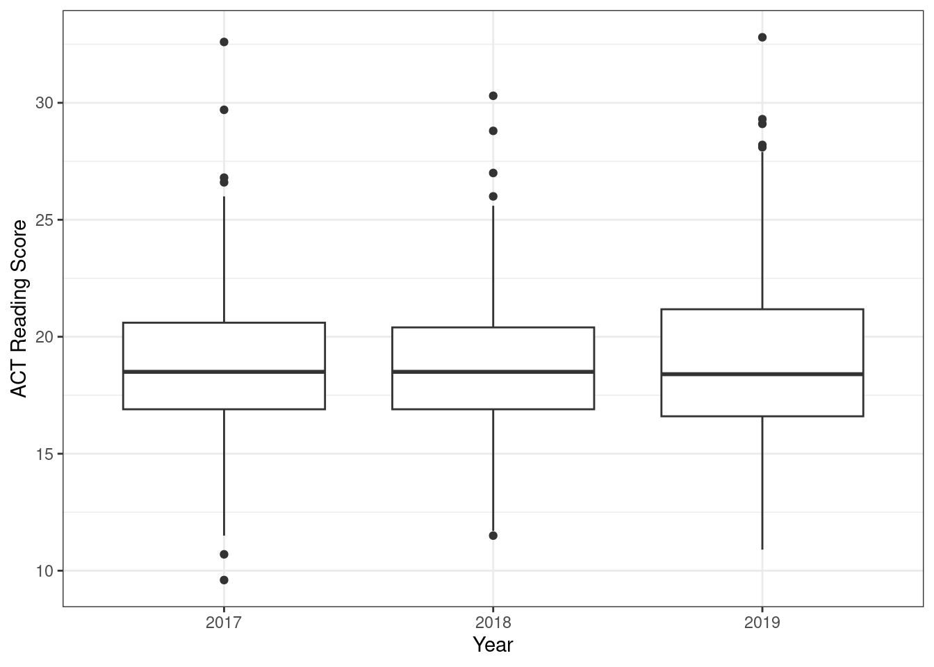
ACT Writing
ggplot(dataset, aes(x = as.factor(year), y = act_writing)) +
  geom_boxplot() +
  labs(x = "Year", y = "ACT Writing Score") +
  theme_bw()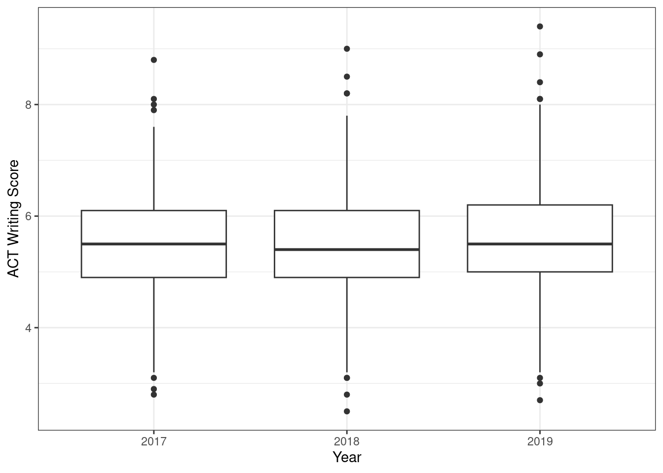
SAT
ggplot(dataset, aes(x = as.factor(year), y = sat_erw)) +
  geom_boxplot() +
  labs(x = "Year", y = "SAT ERW Score") +
  theme_bw()
Correlations
I now look at the main focus of the analysis: the correlation between EOC scores and ACT/SAT scores. We can see that with the possible exception of the SAT correlation, the relationships between EOC scores and the national tests are well approximated by a simple linear model. It looks like the slope of the SAT ~ EOC line would be steeper if not for some high-leverage data points with higher EOC scores and lower SAT scores.
Confirming the impression that scores have been consistent over time, we see through regression analysis that the year variable is not statistically significant in any of the models.
EOC and SAT
Regression
eoc_sat_model <- lm(sat_erw ~ eoc_english + year, data = dataset)| Variable | Coefficient | Standard Error |
|---|---|---|
| EOC | 64.0473544 | 1.7957044 |
| Year | 1.7458006 | 1.0661245 |
| Coefficient | -3175.6908214 | 2151.5119343 |
For a one point increase on the EOC, we can expect to add an average of 64.05 points on the SAT ERW section.
Visualization
ggplot(dataset, aes(x = eoc_english, y = sat_erw)) +
  geom_point(alpha = 0.25) +
  geom_smooth(method = "lm", formula = y ~ x) +
  labs(x = "EOC English Score", y = "SAT ERW Score") +
  theme_bw()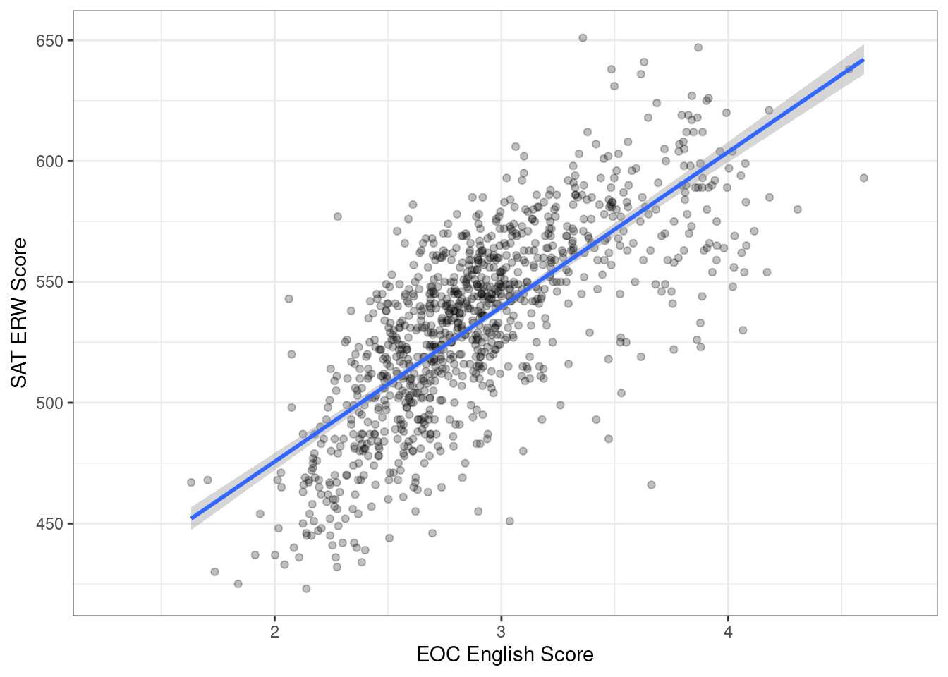
EOC and ACT English
Regression
eoc_act_english_model <- lm(act_english ~ eoc_english + year, data = dataset)| Variable | Coefficient | Standard Error |
|---|---|---|
| EOC | 4.7707492 | 0.0621818 |
| Year | -0.2844032 | 0.0444428 |
| Coefficient | 576.5974144 | 89.6889905 |
For a one point increase on the EOC, we can expect to add an average of 4.77 points on the ACT English section.
Visualization
ggplot(dataset, aes(x = eoc_english, y = act_english)) +
  geom_point(alpha = 0.25) +
  geom_smooth(method = "lm", formula = y ~ x) +
  labs(x = "EOC English Score", y = "ACT English Score") +
  theme_bw()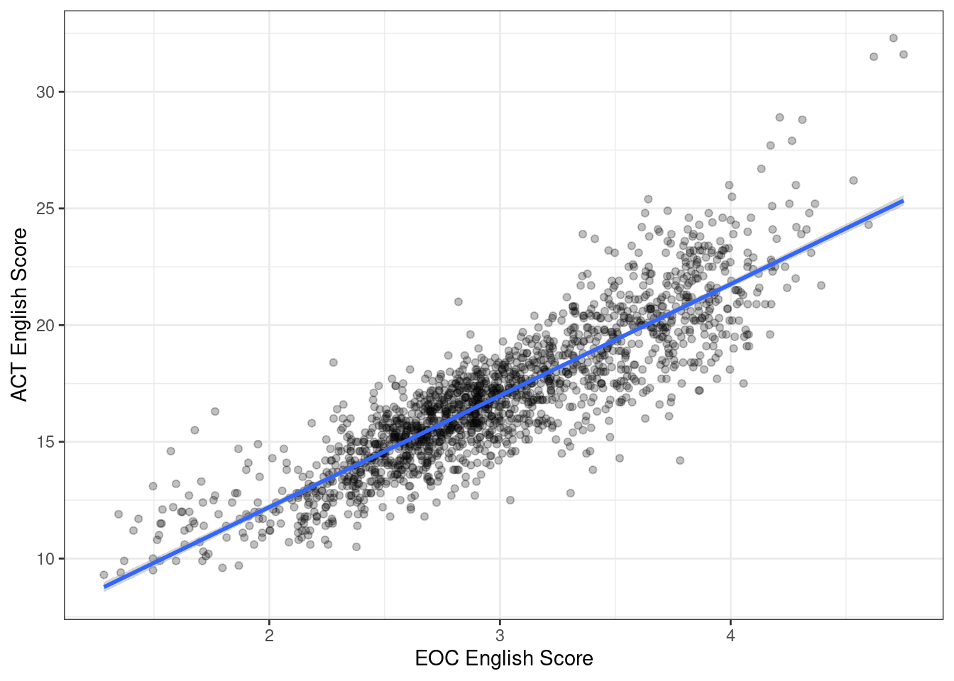
EOC and ACT Reading
Regression
eoc_act_reading_model <- lm(act_reading ~ eoc_english + year, data = dataset)| Variable | Coefficient | Standard Error |
|---|---|---|
| EOC | 4.7312901 | 0.0577885 |
| Year | 0.1176989 | 0.0413028 |
| Coefficient | -232.8635509 | 83.3521659 |
For a one point increase on the EOC, we can expect to add an average of 4.73 points on the ACT reading section.
Visualization
ggplot(dataset, aes(x = eoc_english, y = act_reading)) +
  geom_point(alpha = 0.25) +
  geom_smooth(method = "lm", formula = y ~ x) +
  labs(x = "EOC English Score", y = "ACT Reading Score") +
  theme_bw()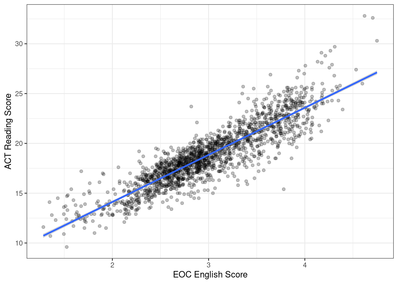
EOC and ACT Writing
Regression
eoc_act_writing_model <- lm(act_writing ~ eoc_english + year, data = dataset)| Variable | Coefficient | Standard Error |
|---|---|---|
| EOC | 1.282358 | 0.0214718 |
| Year | 0.0549683 | 0.0152415 |
| Coefficient | -109.2267805 | 30.7588753 |
For a one point increase on the EOC, we can expect to add an average of 1.28 points on the ACT writing section.
Visualization
ggplot(dataset, aes(x = eoc_english, y = act_writing)) +
  geom_point(alpha = 0.25) +
  geom_smooth(method = "lm", formula = y ~ x) +
  labs(x = "EOC English Score", y = "ACT Writing Score") +
  theme_bw()
Conclusion
It is very clear both visually and statistically that EOC English scores are highly correlated with the verbal sections in the ACT and SAT. The year the exam was taken does not meaningfully impact the relationship, because scores are remarkably stable over the time period in question.