library(dplyr)
library(ggplot2)
library(readxl)Reading Critical Role Stats: Natural 1s and 20s
r
tidyverse
data cleaning
d&d
The goal of this project is to demonstrate loading and cleaning a dataset from Crit Role Stats. They collect data on every dice roll in Critical Role, but the data can be very messy. It’s entered by hand by volunteers, and in general D&D games can be very complicated so the data doesn’t always fall neatly into tidy datasets. After ingesting and cleaning the data, I will use it to determine which episodes had the most and fewest natural 1s and natural 20s, and which had the highest and lowest proportions of each. This is only one application of Crit Role Stats, but there are limitless possibilities for gaining insights from their data.
In this project, I look specifically at data from Campaign 1: Vox Machina.
Data Import
First download the All Rolls spreadsheet from Critical Role Stats. I have this file in my .gitignore because the file is too big to load to GitHub.
Then read it in:
rolls <- read_excel(
  "all-rolls.xlsx",
  sheet = "All Episodes",
  skip = 1,
  col_names = c(
    "episode",
    "time",
    "character",
    "type_of_roll",
    "total_value",
    "natural_value",
    "crit",
    "damage",
    "num_kills",
    "notes"
  ),
  col_types = "text"
)
Data Cleaning
Let’s sanitize the natural_value column for invalid values. I’ll first examine the unique values to determine which ones need to be coerced to NA.
unique(rolls$natural_value) [1] "18.0" "2.0" "3.0" "15.0" "17.0" "6.0" "7.0"
[8] "8.0" "12.0" "13.0" "1.0" "Unknown" "4.0" NA
[15] "20.0" "10.0" "16.0" "14.0" "11.0" "9.0" "19.0"
[22] "5.0" "23.0" "21.0" "0.0" "--" "22.0" "unknown"
[29] "Unkown" "26.0" "24.0" "-4.0" "25.0" "-1.0" "Uknown" There are a few variations of the spelling of “unknown” to account for, along with “–” which is obviously NA. Moreover, there are values below 1 and above 20.
Because I’m only concerned with looking at the number and proportion of natural 20s and natural 1s, I’m going to leave in the rows that have natural roll values reported outside of the 1 to 20 range because they still factor into the total number of rolls and they count as non-critical, so we know all that we need to know from those data points.
na_values <- c(
  "Unknown", "unknown", "Unkown", "Uknown", "--"
)
rolls <- rolls |>
  filter(!(natural_value %in% na_values)) |>
  filter(!is.na(natural_value))
Next, I want to filter out rolls that are not d20 rolls. I do this manually, looking at the unique values of type_of_roll and pulling out all those that are not attack rolls, ability checks, or saving throws, or other values where it’s indicated that the roll is a d20. I go ahead and filter out the 5 NA values:
rolls <- filter(rolls, !is.na(type_of_roll))I will go through the types of rolls that are at all ambiguous:
Unknown: There are three rows with unknown roll type. Two of them have unknown natural value, so they are already omitted. The last one is known to be either a deception or persuasion roll (it’s common that we don’t know which of those two), so it stays in the data set.Alchemy: Keyleth makes two alchemy kit checks, which are d20 rollsBeardandBeard Check: These are d100 rolls that Grog makes to see if he grows a beard using his Belt of Dwarven Kind. They are omitted from the data set.Determine Focus: It’s not clear what this is for. They’re both Grog rolls from episode 33, with values of 15 and 11. I’m going to guess that they’re d20 rolls.Divine Intervention: This is a d100 roll, so is omitted from the data set.Disappointment: I initially assumed that this would be omitted, but it is specifically recorded as a natural 20, so it’s obviously a d20 roll that needs to stay in the data set.Fart.: Same asDisappointment, this is a strange one but it’s a natural 20, so it stays.Inspiration: Inspiration dice are never d20s, so they’re removed from the data set.Missile Snare: This is a d10 roll, so it’s omitted.Musical Taste: Watching the stream, this is in fact a d20 rollNo reason.: This is reported as a natural 1, so it stays.Other: It looks like there are a couple that are clearly d20 rolls, but most of them are either ambiguous or clearly not d20 rolls. I will lose a bit of data but I’m going to omit this category.Spell Effect: It’s not at all clear what this roll was, other than that it was associated with a Dimension Door spell from Scanlan. I suspect it was a d20 roll but it could have been anything, so I’m going to leave it out.Test Roll: There is only one of these, and it is reported as a natural 1. So it stays in.Trajectory: I can’t tell at all what this is referring to, so I’m leaving it out.
non_d20 <- c(
  "Beard",
  "Beard Check",
  "Cutting Words",
  "d100",
  "Damage",
  "Divine Intervention",
  "Inspiration",
  "Missile Snare",
  "Other",
  "Spell Effect",
  "Trajectory"
)

rolls <- filter(rolls, !(type_of_roll %in% non_d20))
I also want to sanitize a few episode numbers:
rolls$episode[rolls$episode %in% c("31 p1", "31 p2")] <- 31
rolls$episode[rolls$episode %in% c("33 p1", "33 p2")] <- 33
rolls$episode[rolls$episode %in% c("35 p1", "35 p2")] <- 35
rolls$episode <- as.integer(rolls$episode)
Analysis: Natural 1s and 20s
I want to see which episode had the most natural 20s and which had the most natural 1s, as well as which episodes had the highest proportions of natural 20s and natural 1s.
crits <-
  rolls |>
  mutate(natural_value = as.numeric(natural_value)) |>
  group_by(episode) |>
  summarize(
    n_rolls = n(),
    nat_20 = sum(natural_value == 20),
    nat_1 = sum(natural_value == 1)
  ) |>
  mutate(nat_20_prop = nat_20 / n_rolls,
         nat_1_prop = nat_1 / n_rolls)
So which episode has the most natural 20s? Since the episode column is in order, we can simply get the index of the row. This code chunk uses base R, without tidyverse functions, because it’s more terse and less verbose. Chunks lower down use tidyverse functions where they are simpler and more concise to use.
episodes <- tibble(
  label = c(
    "Fewest Natural 1s",
    "Lowest Natural 1 Proportion",
    "Most Natural 1s",
    "Highest Natural 1 Proportion",
    "Fewest Natural 20s",
    "Lowest Natural 20 Proportion",
    "Most Natural 20s",
    "Highest Natural 20 Proportion"
  )
)
episodes[, c("episode",
  "n_rolls",
  "nat_1",
  "nat_1_prop",
  "nat_20",
  "nat_20_prop")] <-  crits[c(
  which.min(crits$nat_1),
  which.min(crits$nat_1_prop),
  which.max(crits$nat_1),
  which.max(crits$nat_1_prop),
  which.min(crits$nat_20),
  which.min(crits$nat_20_prop),
  which.max(crits$nat_20),
  which.max(crits$nat_20_prop)
),
c("episode",
  "n_rolls",
  "nat_1",
  "nat_1_prop",
  "nat_20",
  "nat_20_prop")]

episodes
# A tibble: 8 × 7
label episode n_rolls nat_1 nat_1_prop nat_20 nat_20_prop
<chr> <int> <int> <int> <dbl> <int> <dbl>
1 Fewest Natural 1s 18 69 0 0 4 0.0580
2 Lowest Natural 1 Proporti… 18 69 0 0 4 0.0580
3 Most Natural 1s 111 115 12 0.104 10 0.0870
4 Highest Natural 1 Proport… 57 14 3 0.214 0 0
5 Fewest Natural 20s 56 24 1 0.0417 0 0
6 Lowest Natural 20 Proport… 56 24 1 0.0417 0 0
7 Most Natural 20s 7 131 2 0.0153 16 0.122
8 Highest Natural 20 Propor… 73 5 0 0 1 0.2 Episodes with No Natural 1s
no_nat_1s <- crits |>
  slice_min(nat_1, n = 1) |>
  select(episode, n_rolls, nat_1)
There are 13 episodes with no natural 1s:
no_nat_1s# A tibble: 13 × 3
episode n_rolls nat_1
<int> <int> <int>
1 18 69 0
2 26 42 0
3 37 86 0
4 41 66 0
5 45 31 0
6 46 99 0
7 47 44 0
8 73 5 0
9 74 39 0
10 89 22 0
11 91 19 0
12 97 40 0
13 101 52 0Episodes with No Natural 20s
no_nat_20s <- crits |>
  slice_min(nat_20, n = 1) |>
  select(episode, n_rolls, nat_20)
There are 3 episodes with no natural 20s:
no_nat_20s# A tibble: 3 × 3
episode n_rolls nat_20
<int> <int> <int>
1 56 24 0
2 57 14 0
3 74 39 0It is pretty interesting that there are so many more episodes without natural 1s than without natural 20s. This is possibly due to players not actually announcing all of their natural 1s. In many cases, the players will just indicate that they’ve failed the roll without specifying that they rolled a 1. In these instances, Crit Role Stats cannot record that roll, so we lose data and get more skewed data.
Lowest Proportion of Natural 1s and 20s
We know that the episodes with the lowest proportion of natural 1s and 20s will be those without any natural 1s or 20s at all. But that’s not especially interesting. What are the episodes with the lowest proportion of crits among those that had at least one?
crits |>
  filter(nat_1 > 0) |>
  slice_min(nat_1_prop, n = 1) |>
  union(crits |>
          filter(nat_20 > 0) |>
          slice_min(nat_20_prop, n = 1))
# A tibble: 2 × 6
episode n_rolls nat_20 nat_1 nat_20_prop nat_1_prop
<int> <int> <int> <int> <dbl> <dbl>
1 98 86 11 1 0.128 0.0116
2 20 58 1 5 0.0172 0.0862In both instances, the proportions are between 1 and 2 percent, considerably lower than the average proportion of 5%.
Most Natural 1s and 20s
crits |>
  slice_max(nat_1, n = 1) |>
  union(slice_max(crits, nat_20, n = 1)) |>
  union(slice_max(crits, nat_1_prop, n = 1)) |>
  union(slice_max(crits, nat_20_prop, n = 1))
# A tibble: 5 × 6
episode n_rolls nat_20 nat_1 nat_20_prop nat_1_prop
<int> <int> <int> <int> <dbl> <dbl>
1 111 115 10 12 0.0870 0.104
2 7 131 16 2 0.122 0.0153
3 100 152 16 6 0.105 0.0395
4 57 14 0 3 0 0.214
5 73 5 1 0 0.2 0 There are two episodes tied for most natural 20s – episodes 7 and 100 each have 16 natural 20s. However, they have very different numbers of total rolls, leading to very different proportions. For proportions, unsurprisingly the episodes with the highest proportions of crits are those with relatively few total rolls. Episode 57 had 3 natural 1s, but only 14 total rolls, and episode 73 only had 5 total rolls, of which 1 was a natural 20.
Visualizations
Finally, we can visualize this data in a number of different ways. However, given that rolls are inherently random, we should expect the visualizations to be fairly random as well.
Natural 1s by Episode
ggplot(crits, aes(x = episode, y = nat_1)) +
  geom_line() +
  labs(x = "Episode Number", y = "Natural 1s") +
  theme_bw()
Natural 20s by Episode
ggplot(crits, aes(x = episode, y = nat_20)) +
  geom_line() +
  labs(x = "Episode Number", y = "Natural 20s") +
  theme_bw()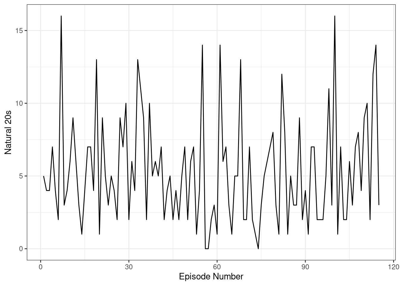
Natural 1 Proportion by Episode
ggplot(crits, aes(x = episode, y = nat_1_prop)) +
  geom_line() +
  labs(x = "Episode Number", y = "Proportion Natural 1s") +
  theme_bw()
Natural 20 Proportion by Episode
ggplot(crits, aes(x = episode, y = nat_20_prop)) +
  geom_line() +
  labs(x = "Episode Number", y = "Proportion Natural 20s") +
  theme_bw()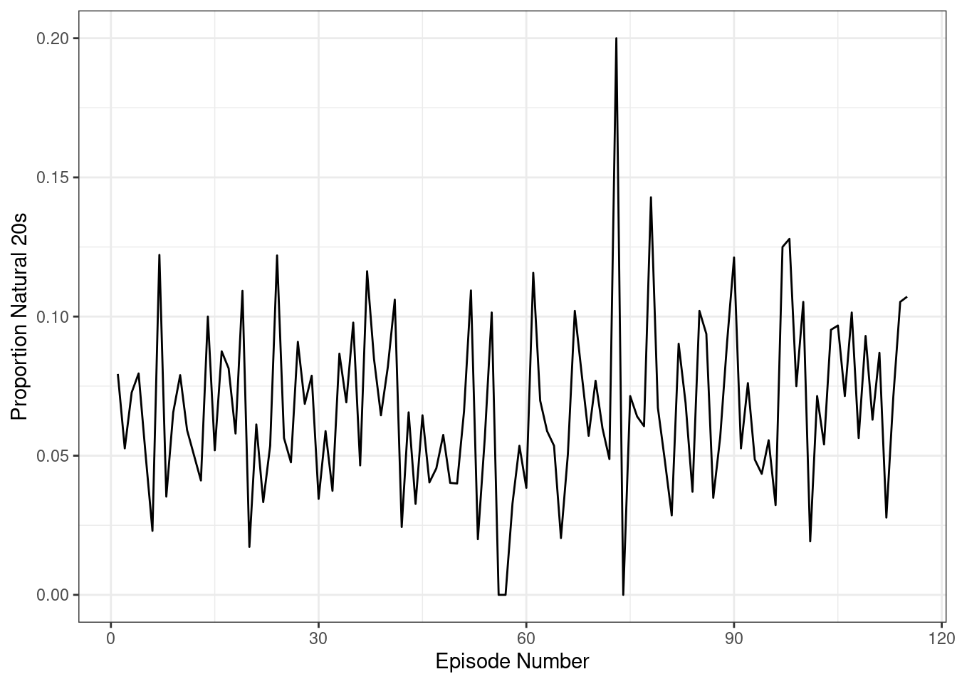
Total Rolls by Episode
We may expect to see cyclical patterns in the number of total rolls, following the various arcs of the campaign.
ggplot(crits, aes(x = episode, y = n_rolls)) +
  geom_line() +
  labs(x = "Episode Number", y = "Total Rolls") +
  theme_bw()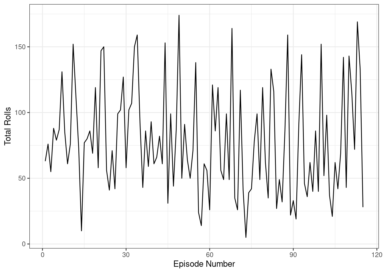
We don’t see the clearest pattern of total rolls aligning with major arcs, but we do see a bit of a pattern of a few episodes with lower total rolls followed by one or two with many more total rolls.
Total Rolls Frequency Chart
We may also be interested to see the overall distribution of total rolls.
Average number of rolls:
mean(crits$n_rolls)[1] 78.08772ggplot(crits, aes(x = n_rolls)) +
geom_bar() +
geom_vline(xintercept = mean(crits$n_rolls), linewidth = 1.5, color = "red") +
theme_bw()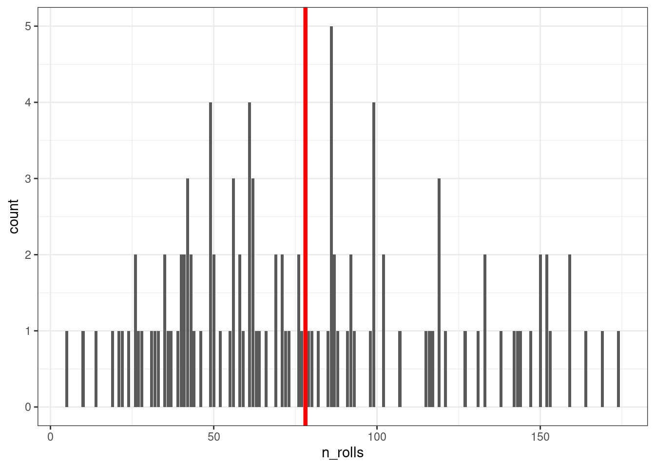
Conclusion
The most informative result from this analysis is determining the episodes with the lowest and highest proportion of critical rolls. The absolute numbers are predictably highly influenced by the total number of rolls in each episode. In the episodes with relatively few total rolls, we see the highest proportion of natural 1s and 20s. The plots of critical rolls over time are not especially informative, as they represent multiple trials of random processes, so the visualizations are fairly random. This was a useful exercise in data importing, cleaning, and manipulating, and illustrates the importance of substantive knowledge of the data set you’re working with. Without extensive knowledge of Dungeons and Dragons and how Critical Role is played and presented, it would be very difficult to determine which types of rolls to include and how to filter out the unusual array of roll type. I am definitely looking forward to revisiting Crit Role Stats in future projects.