library(leaflet)
library(sf)
library(tidyverse)Plotting Geospatial Data: Boston Housing Violations
r
ggplot2
leaflet
geospatial
In this post, I will be working with the sf package to read in geospatial data to plot the 2020 census block groups of Boston, and use ggplot2 and leaflet to overlay a plot of property and housing violations. This is a simple post but I will come back to the principles and process described here in a future project.
Geospatial Data with sf
I am using data from Boston’s “Analyze Boston” project, which provides open access to huge amounts of city data. The first one that I’m using is 2020 census block groups in Boston, which I downloaded in GeoJSON format here. We can read this in with sf::st_read():
block_groups <- st_read("boston_block_groups.geojson", quiet = TRUE)We can take a look at the data using the sf-specific print() method.
print(block_groups, n = 3)Simple feature collection with 581 features and 14 fields
Geometry type: MULTIPOLYGON
Dimension: XY
Bounding box: xmin: -71.19125 ymin: 42.22792 xmax: -70.9201 ymax: 42.40494
Geodetic CRS: WGS 84
First 3 features:
geoid20 countyfp20 namelsad20 statefp20 bgid tractce20 intptlat20
1 250250406001 025 Block Group 1 25 0406001 040600 +42.3833695
2 250250511011 025 Block Group 1 25 0511011 051101 +42.3882285
3 250250511014 025 Block Group 4 25 0511014 051101 +42.3913407
funcstat20 intptlon20 blkgrpce20 mtfcc20 aland20 awater20 objectid
1 S -071.0707743 1 G5030 1265377 413598 1
2 S -071.0046816 1 G5030 220626 0 2
3 S -071.0020343 4 G5030 227071 270 3
geometry
1 MULTIPOLYGON (((-71.08097 4...
2 MULTIPOLYGON (((-71.01084 4...
3 MULTIPOLYGON (((-71.00629 4...The output tells me that there are 581 “features”, i.e. records and 14 “fields,” or non-spatial attributes. The dimensions given are XY so we know that it maps to a simple two-dimensional coordinate plane. We are also given the bounding box and the coordinate reference system, WGS 84. Because we’re working in a small geographic area where the curvature of the earth can largely be disregarded, that’s not something we really need to worry about here.
We can use the plot() method for the sf data frame to easily render a very nice plot of the data. This one shows it colored simply by the block group ID (geoid20).
plot(block_groups[1])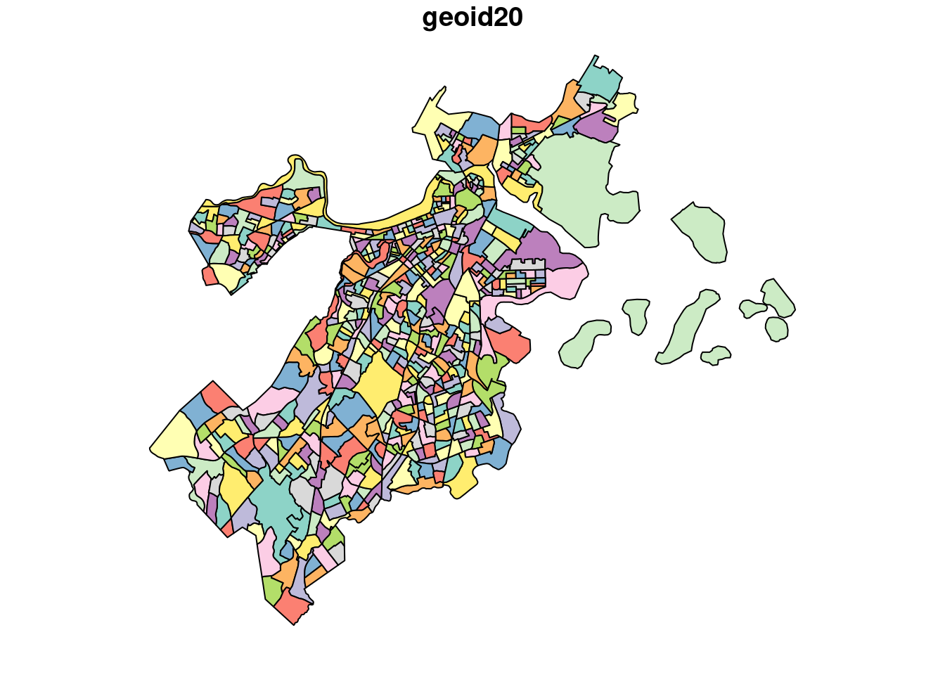
We can also use ggplot2 to plot this using geom_sf() (I like theme_bw() for maps):
ggplot(block_groups) +
  geom_sf() +
  theme_bw()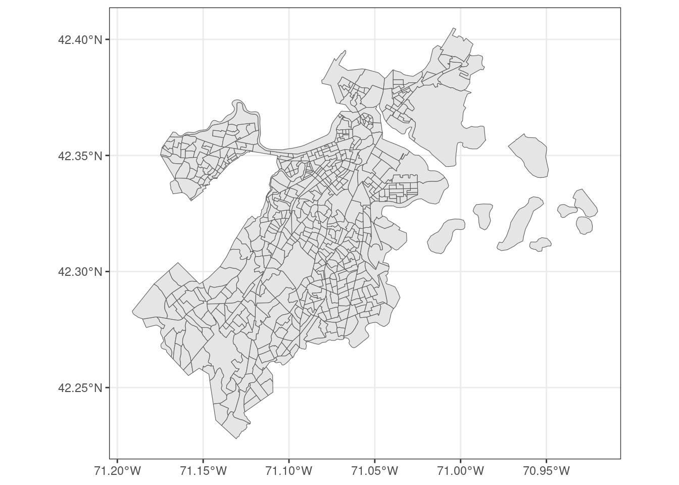
That gives us nice axis labels by default. Note that this does not color the polygons, and trying to add a fill aesthetic doesn’t really work:
ggplot(block_groups, aes(fill = geoid20)) +
  geom_sf()
So that’s off the table as far as quick and easy plots go. It doesn’t really make sense to color by ID other than for appearances, and ggplot2 should handle fills more easily when there isn’t a distinct value for every single feature.
Aside from ggplot2, I could also use leaflet to plot these census block groups.
leaflet(block_groups) |>
  addTiles() |>
  addPolygons(weight = 1)
Property Violations
The second dataset I’m using is building and property violations, which I downloaded here. Here’s a quick look:
violations <- read_csv("violations.csv")
glimpse(violations)
Rows: 14,530
Columns: 23
$ case_no <chr> "V700667", "V700258", "V700254", "V700251", "V700239"…
$ status_dttm <dttm> 2023-09-11 09:40:06, 2023-09-08 15:31:32, 2023-09-08…
$ status <chr> "Open", "Open", "Open", "Open", "Open", "Open", "Open…
$ code <chr> "102.8", "102.8", "102.8", "102.8", "102.8", "116", "…
$ value <chr> "N/A", "N/A", "N/A", "N/A", "N/A", "N/A", "N/A", "N/A…
$ description <chr> "Maintenance", "Maintenance", "Maintenance", "Mainten…
$ violation_stno <chr> "14", "50", "33", "42", "11", "29", "93", "342", "115…
$ violation_sthigh <chr> NA, NA, NA, NA, NA, "31", NA, NA, NA, "109", "154", N…
$ violation_street <chr> "Wadsworth", "Ashford", "Pratt", "Pratt", "Nott", "La…
$ violation_suffix <chr> "ST", "ST", "ST", "ST", "ST", "ST", "ST", "ST", "ST",…
$ violation_city <chr> "Allston", "Allston", "Allston", "Allston", "Hyde Par…
$ violation_state <chr> "MA", "MA", "MA", "MA", "MA", "MA", "MA", "MA", "MA",…
$ violation_zip <chr> "02134", "02134", "02134", "02134", "02136", "02119",…
$ ward <chr> "21", "21", "21", "21", "18", "09", "05", "01", "06",…
$ contact_addr1 <chr> "945 RANDOLPH ST", "34 CEDAR STREET", "28 BROOK ST"…
$ contact_addr2 <chr> NA, NA, NA, NA, NA, NA, NA, NA, NA, "109 STATE STREET…
$ contact_city <chr> "CANTON", "WELLESLEY", "BRIGHTON", "ALLSTON", "BOSTON…
$ contact_state <chr> "MA", "MA", "MA", "MA", "MA", "MA", "MA", "MA", "MA",…
$ contact_zip <chr> "02021", "02481", "02135", "02134", "02110", "02120",…
$ sam_id <dbl> 141274, 5173, 112504, 112514, 104194, 83655, 12466, 3…
$ latitude <dbl> 42.35518, 42.35471, 42.35490, 42.35536, 42.25463, 42.…
$ longitude <dbl> -71.12613, -71.12643, -71.12842, -71.12769, -71.11909…
$ location <chr> "(42.355179609050516, -71.12613060638347)", "(42.3547…It is very handy that this data set already includes latitude and longitude. If it didn’t, we would have to geocode each address using something like the Nominatim API.
Because ggplot2 allows each layer to have its own data, we can easily overlay the points from the violations data frame onto the polygons given by block_groups without having to worry about joining the data frames. I add on coord_sf() so that I can specify the coordinate reference system. Again, we’re working with such a small geographic area that we don’t need to worry too much about distortions because of the curvature of the earth, but it’s better to be thorough.
ggplot() +
  geom_sf(data = block_groups) +
  geom_point(
    data = violations,
    mapping = aes(x = longitude, y = latitude),
    size = 0.05,
    alpha = 0.1
  ) +
  coord_sf(crs = st_crs(block_groups)) +
  theme_bw()
What jumps out in my mind when I look at that chart is the presence of large census block groups that have zero violations. My guess is that these are parks but I would want to confirm this.
We could again use leaflet to plot this, which would also give us the benefit of seeing exactly what those large, no-violation census block groups are.
leaflet(block_groups) |>
  addTiles() |>
  addPolygons(weight = 1) |>
  addCircleMarkers(
    lng = violations$longitude,
    lat = violations$latitude,
    stroke = FALSE,
    color = "black",
    radius = 1,
    fillOpacity = 0.5
  )
That looks pretty good, and those large blocks are in fact parks, as well as the airport and some outlying islands.
That’s it! As long as you have nice, clean data, the plotting is really pretty straightforward. I’m lucky that the violations data set was so conveniently organized and tidy, which makes it a good demonstration.