The Weight of Advantage and Disadvantage in Dungeons & Dragons

How much does advantage help, and how much does disadvantage hurt?

suppressPackageStartupMessages(library(ggplot2))

In Dungeons & Dragons 5th Edition, player actions are generally resolved by rolling a 20 sided die (a d20) and adding a relevant modifier. The Game Master may allow a player to roll with either advantage or disadvantage. In both cases, you roll the d20 twice. With advantage, you take the higher of the two values, and with disadvantage you take the lower. Now the average roll of a d20 is 10.5:

mean(1:20)

[1] 10.5

But how do advantage and disadvantage affect that?

Because this analysis involves random sampling, I use set.seed() to ensure replicability:

set.seed(2023)

For both of these, we start by making repeated pairs of draws from a uniform distribution from 1 to 20. For advantage, we take the maximum, and for disadvantage we take the minimum. I will be using a total of 1 million pairs of draws, just to make sure we really get the law of large numbers working for us.

n <- 1e6
draws <- matrix(0, nrow = n, ncol = 4)
colnames(draws) <- c("draw_1", "draw_2", "advantage", "disadvantage")
draws[, c("draw_1", "draw_2")] <- replicate(
  n = n, 
  sample(1:20, size = 2, replace = TRUE)
)

Next, I take the maximum and minimum values of each pair for the advantage and disadvantage columns, respectively. Here, apply() takes an input matrix, in this case the columns draw_1 and draw_2 from the draws matrix. The second argument, 1, tells it to apply the function, max() over the rows of the input matrix. That is, for each row, apply the max() function. The MARGIN argument of 1 indicates rows because in matrix subsetting in R, the first term indicates the row and the second term indicates the column, i.e. draws[5,10] indicates the 5th row of the 10th column.

draws[, "advantage"] <- apply(draws[, 1:2], 1, max)
draws[, "disadvantage"] <- apply(draws[, 1:2], 1, min)

We can plot the frequency distributions for these. For a standard roll, i.e. just the first draw, we should expect a roughly uniform distribution across all values.

ggplot(data.frame(draws), aes(x = draw_1)) + 
  geom_bar(col = "black") + 
  theme_bw()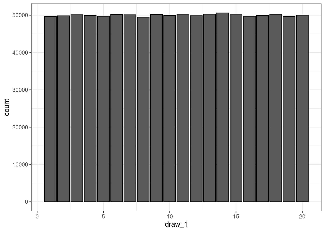

Because of the very large number of rolls, we do see the distribution has mostly converged to the expected uniform distribution of the population.

For advantage:

ggplot(data.frame(draws), aes(x = advantage)) + 
  geom_bar(col = "black") + 
  theme_bw()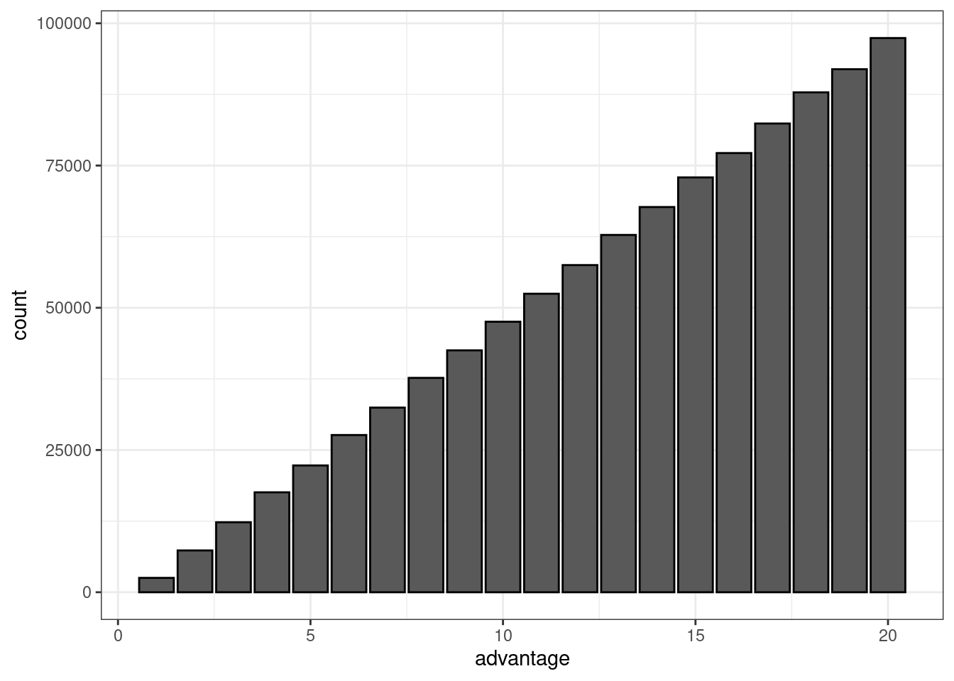

In this case, we have a PMF that is linear in \(x\). The PMF thus resembles \(P(X=x) = a+bx : 1 \leq x \leq 20\), where the probability of \(X=x\) is greater and greater for each increasing value of \(x\). Solving a simple system of equations using the \(P(X=1)\) and \(P(X=20)\), I have calculated \(a\approx-0.0025\) and \(b\approx0.005\). This could also be solved using linear regression. To do that, I get the proportions of roll results from the advantage rolls and regress that proportion on the roll value.

df <- data.frame(table(draws[, "advantage"]) / n)
colnames(df) <- c("x", "p_x")
df$x <- as.numeric(df$x)  # `table` produces a factor for this value
lm(p_x ~ x, data = df)

Call:
lm(formula = p_x ~ x, data = df)

Coefficients:
(Intercept)            x  
  -0.002506     0.005001  

For disadvantage:

ggplot(data.frame(draws), aes(x = disadvantage)) + 
  geom_bar(col = "black") + 
  theme_bw()

We can repeat the process used for advantage to calculate the parameters for the disadvantage distribution:

df <- data.frame(table(draws[, "disadvantage"]) / n)
colnames(df) <- c("x", "p_x")
df$x <- as.numeric(df$x)
lm(p_x ~ x, data = df)

Call:
lm(formula = p_x ~ x, data = df)

Coefficients:
(Intercept)            x  
   0.102383    -0.004989  

---

Then I compute the mean and standard deviation of each:

results <- data.frame(
  type = c("Standard", "Advantage", "Disadvantage"),
  mean = c(mean(draws[, "draw_1"]), mean(draws[, "advantage"]), mean(draws[, "disadvantage"])),
  sd = c(sd(draws[, "draw_1"]), sd(draws[, "advantage"]), sd(draws[, "disadvantage"]))
)

results

          type     mean       sd
1     Standard 10.50629 5.761983
2    Advantage 13.82537 4.705335
3 Disadvantage  7.18243 4.711922

It’s pretty clear that advantage and disadvantage substantially affect the average result. We can quantify that difference using a t-test to measure difference in means. For advantage:

t.test(draws[, "advantage"], draws[, "draw_1"])

    Welch Two Sample t-test

data:  draws[, "advantage"] and draws[, "draw_1"]
t = 446.17, df = 1923180, p-value < 2.2e-16
alternative hypothesis: true difference in means is not equal to 0
95 percent confidence interval:
 3.304502 3.333662
sample estimates:
mean of x mean of y 
 13.82537  10.50629 

We get a 95% confidence interval of (3.31, 3.34), and it makes sense that we would get such a tight interval given an n of 1,000,000.

For disadvantage:

t.test(draws[, "draw_1"], draws[, "disadvantage"])

    Welch Two Sample t-test

data:  draws[, "draw_1"] and draws[, "disadvantage"]
t = 446.56, df = 1924170, p-value < 2.2e-16
alternative hypothesis: true difference in means is not equal to 0
95 percent confidence interval:
 3.309267 3.338445
sample estimates:
mean of x mean of y 
 10.50629   7.18243 

So next time, do your best to get advantage however you can, and avoid disadvantage at all costs. The probability of getting a natural 20 with advantage nearly double compared to a standard roll, and the same goes for getting a natural 1 with disadvantage. Happy gaming!